- Set up your SAS environment (see § 2.3.1)
- Extract an image (in sky coordinates in this example;
extraction in detector - DET[XY] - coordinates is possible as well)
      evselect table=PN.evt:EVENTS imagebinning=binSize \
        imageset=PNimage.fits withimageset=yes \
        xcolumn=X ycolumn=Y ximagebinsize=80 yimagebinsize=80
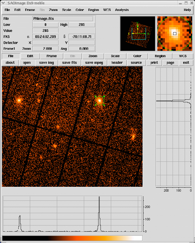
- Display the image
imgdisplay withimagefile=true imagefile=PNimage.fits
- Select the region, from which the light curve shall be
accumulated, using the Region/Circle in ds9 (see figure 35).
Figure 35:
ds9 main window. A circular region (green circle) has been defined using the highlighted menu.
 |
- Double-click with the cursor on the defined region. A window
pops up, showing the properties of the region (figure 36). Write
down the coordinates of the Center (25910.5, 25870.5)
and the Radius (400).
Figure 36:
Selection region properties window, pop'd-up by double-clicking on the region in the main ds9 window.
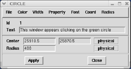 |
Units of sky coordinates (X,Y) are 0.05 arcsec, hence the radius in our example is 20 arcsec.
- Be aware: if you are interested in very short time periods,
such as they appear in pulsars of cataclysmic variables, you
have to perform a barycentric correction. This means that the
arrival time of a photon is shifted as is it would have been
detected at the barycenter of the solar system (the center of
mass) instead at the position of the satellite. In this way,
the data are comparable. The SAS task barycen performs this
correction. It is advisable first to copy the event list
since the TIME column of the event list is directly
overwritten by the barycentric corrected times
       cp PN.evt PN_evlist.fit

       barycen table=PN_evlist.fit
- Now you can extract a source+background light curve, using all
the selection expressions defined so far. In the example, the
binsize is 100 seconds. Please take into account that operating
with non-synchronous time series can introduce artifacts when
they are added or subtracted by programmes such as the ftools
lcmath. From SAS v8.0 onwards, there is no need to
do so, since by default the start time is set to the beginning
of the exposure. You can override this by using the parameter
timemin and timemax.
      evselect table=PN.evt energycolumn=PI \
        expression='#XMMEA_EP&&(PATTERN<=4)&& \
        ((X,Y) IN circle(25910.5,25870.5,400))&&(PI in [200:10000])' \
        withrateset=yes rateset="light_curve.fits" timebinsize=100 \
        maketimecolumn=yes makeratecolumn=yes timemin=126991800 \
        timemax=130000000
The parameter makeratecolumn=yes produces a light curve in count
rates (with errors). Otherwise the light curve is produced in counts (with errors).
- Repeat step 4. to 6. above to determine the region, from which
the background light curve is to be extracted. It will be assumed
in what follows that the extraction region correspond to an
annulus, centered in (25910.5,25870.5) and with inner and
outer radii 1000 and 2000 pixels, respectively.
- Extract a background light curve, using all the selection
expressions defined so far, and the same binsize (100 seconds) and
energy range as for the source+background light curve
      evselect table=PN.evt energycolumn=PI \
        expression='#XMMEA_EP&&(PATTERN<=4)&& \
        ((X,Y) IN annulus(25910.5,25870.5,1000,2000)) \
        && (PI in [200:10000])' \
        withrateset=yes rateset="light_curve_background.fits" \
        timebinsize=100 \
        maketimecolumn=yes makeratecolumn=yes \
        timemin=126991800 timemax=130000000
The light curves are OGIP-complaint, and therefore analyzable with
standard XRONOS-like (Xronos) LHEASOFT packages.
- However, light curves obtained in such a way should be
corrected to account for a number of effects which can have an
impact in the detection efficiency, like vignetting, bad pixels, PSF variation
and quantum efficiency, as well as to account for time dependent
corrections within a exposure, like dead time and GTIs. Since all these
corrections can differ between source and
background light curves, the background subtraction
has to be done accordingly. The SAS task epiclccorr
performs all of these corrections at once. It
requires as input both light curves (which are
used to establish the binning of the final
corrected background subtracted light curve)
and the event file. A simple command line call:
       epiclccorr srctslist=PN_lightcurve_raw.FIT \
                  eventlist=PN_evlist.FIT \
                  outset=PN_lccorr.fit \
                  bkgtslist=PN1_lc_bck.FIT \
                  withbkgset=yes \
                  applyabsolutecorrections=yes
- Plot the resulting light curves, eg.
dsplot table=PN_lccorr.fit withx=yes x=TIME withy=yes y=RATE
This command will launch the window shown in figure 37.
Figure 37:
xmgrace window, containing the background subtracted exposure corrected light curve.
 |