| Accuracy Level | scheme | description |
| LOW | analytic | the PSF is constructed using a single bi-dimensional Gaussian fit involving energy dependent parameters which are tabulated in the CCF. This mode is a fastest way to compute the PSF but with a very limited accuracy. In particular, it shall not be used for encircled energy calculations. |
| MEDIUM | library | the PSF is constructed from a library of PSF images provided in the CCF. This is meant to be most direct way to access the PSF. A set of images is extracted from the CCF. Interpolations in energy and field angle are performed. Resampling of the extrapolated image is performed to account for mismatches (e.g rotation) between the requested spatial grid and the one at which the PSF image are stored in the CCF. |
| HIGH | analytic | the PSF is constructed using multi-Gaussian fits involving parameters which are tabulated in the CCF. This mode involve a high number of fitting paramteters which provide an accurate description of the core and wings of the PSF. The validity range is limited to energies lower than 5 keV and field angles smaller than 7 arcmin. |
| EXTENDED | analytic | the PSF is constructed using a single one-dimensional King profile. The parameters of the King function are tabulated in terms of energy and off-axis angle in the CCF. This method gives good accuracy but is only relevant for the one-dimensional case. The parameters of the King function have been measured for energies in the full XMM band pass and at off-axis angles upto 12 arc minutes. However, there are gaps in the applicability which are described in Ghizzardi, S., 2001, EPIC-MCT-TN-011. |
The analytical expression use to describe the PSF in the low accuracy mode is
as follows.
![\begin{eqnarray*}
PSF(y, z) &=& 1/(N p^2)\bigl(\\
&&A_1\exp\left[-\left\{(y-A_2...
...4 + (z-C_3)^2/C_5\right\}\right]
(1+C_6\cos(16\phi+C_7))
\bigr)
\end{eqnarray*}](img56.png)
The analytical expression used to describe the PSF in the extended accuracy mode is as follows:
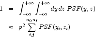
The PSF images provided in the library are sampled on a grid of
(Y_EXTENT,Z_EXTENT) pixels with Y_PIXSZ, Z_PIXSZ pixel size.
These parameters are specified in the CCF components. They are the results
of a trade-off between simulation times and simulation accuracy defined by
field of view and oversampling. The fitting routines are then applied to
these sampled images. Hence, the ![]() coordinates are expressed in sampling
pixel units.
coordinates are expressed in sampling
pixel units.
The CAL provides the PSF in a physical reference frame
![]() in units of mm which is centerd on the
PSF barycenter and whose axes are aligned with the CAL TELCOORD frame.
The conversion
in units of mm which is centerd on the
PSF barycenter and whose axes are aligned with the CAL TELCOORD frame.
The conversion
![]() is
given by:
is
given by:
with
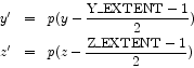
![]() ,
, ![]() ,
, ![]() are the focal length, the off-axis angle and
azimuth of the source position with respect to the EPIC boresight.
are the focal length, the off-axis angle and
azimuth of the source position with respect to the EPIC boresight.
![]() is the sampling pixel size defined in mm in the CCF.
is the sampling pixel size defined in mm in the CCF.
![]() ,
, ![]() and
and ![]() are correction factors which
account for the mirror module field curvature, EPIC defocus, mirror module
tilt with respect to boresight and EPIC decenter with respect to the average
focal point of the mirror modules. Initially these correcting factors will be
set to 0.
are correction factors which
account for the mirror module field curvature, EPIC defocus, mirror module
tilt with respect to boresight and EPIC decenter with respect to the average
focal point of the mirror modules. Initially these correcting factors will be
set to 0.