Calibration Access and Data Handbook

Procedure

The redistribution function of the CCD's is parameterized per CCD and per node. The model is described in [1] with an update described in [2]. It combines the X-ray absorption probability in silicon with an empirical parameterization of the generated charge signal, which is then folded by a Gaussian for noise representation.

The probability $P$ for absorption of a photon in silicon at the depth $x$ is given by

$$\frac{{\rm d}P}{{\rm d}x} = \frac{1}{\tau}\ e^{-x/\tau}\ ,$$ (2)

with the mean absorption length in silicon $\tau$. For a given photon of energy $E$ (in eV), and absorption at $x$, the collected charge $Q$ (in eV) is parameterized with the empirical model

$$Q = \left \{ \begin{array}{ll} 0 & {\rm for}\ Q<T\\ T+(... ...(x/b)^{1/3}} \right ) & {\rm for}\ Q\ge T \end{array} \right.$$ (3)

with a threshold for charge detection $T=50\,{\rm eV}$, and $b=20.95\,{\rm nm}$ being a parameter that defines the scale of the collected charge.

The charge probability density then is

$$\frac{{\rm d}P}{{\rm d}Q} = \frac{{\rm d}P}{{\rm d}x} \frac{{\rm d}x}{{\rm d}Q}\ .$$ (4)

From (3) follows that

$${\rm d}Q = (E-T)\ e^{-(x/b)^{1/3}} \left ( \frac{x}{b} \right )^{-2/3} \frac{1}{3b}\ {\rm d}x\ ,$$ (5)

and hence

$$\frac{{\rm d}P}{{\rm d}Q} = \frac{1}{\tau}\ e^{-x/\tau} \frac{3b}{E-T}\ e^{(x/b)^{1/3}} \left ( \frac{x}{b} \right )^{2/3}$$ (6)

Reforming (3) into

$$\left ( \frac{x}{b} \right )^{1/3} = \ln \frac{E-T}{E-Q}\ ,$$ (7)

allows to eliminate $x$ from (6), and yields

$$\frac{{\rm d}P}{{\rm d}Q} = \frac{3b}{\tau}\ \frac{1}{E-Q}\... ...rac{E-T}{E-Q}\ e^{-\frac{b}{\tau} \ln^3 \frac{E-T}{E-Q} } \ ,$$ (8)

which gives the response probability of an ideal CCD to an incident photon of energy $E$ with the parameters $b$ and $T$ which are specified in the CCF REDIST.

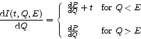
To this function a partial event tail is added that has a constant probability density for all charges less than the incident energy, and zero above:

$$\frac{{\rm d}I(t,Q,E)}{{\rm d}Q} = \left \{ \begin{array}{... ...frac{{\rm d}P}{{\rm d}Q} & {\rm for}\ Q>E \end{array} \right.$$ (9)

$t$ is the differential amplitude of the total fraction of partial events $P_{\rm part}$. It is $t=t(Q)={\tt const}$ and its value is defined from

$$P_{\rm part} = \int_0^E t\: {\rm d}Q = t\ E \ .$$ (10)

$P_{\rm part}$ is parameterized as

$$P_{\rm part} = g \times \left [1 - e^{-c(E-d)}\right ] \times \frac{\tau(E_{\rm ref})}{\tau(E)}$$ (11)

with the parameters $c$, $d$, $g$ and $E_{\rm ref}$, which are specified in the CCF REDIST.

Finally ${\rm d}I(t,Q,E)/{\rm d}Q$ is convolved with a Gaussian to represent the Fano-noise and the amplifier noise. The $\sigma$ (in eV) of this Gaussian can be written as

$$\sigma = \sqrt{FEw + sa^2w^2}\, ,$$ (12)

with Fano factor $F$, mean pair generation energy $w$ (in ${\rm eV/e^-}$), average event size $s$ (in pixels), and amplifier noise $a$ (in electrons).

It has to be noted that the result of the this function, as far as described so far, is in units of energy. In order to be able to compare with data, which are in units of PI, the output of this function has to be converted to PI, taking the relationship between the definition of PI and energy into account.

Note that the Si escape peak is not included in the current model.