XMM-Newton Users Handbook

3.4.4.5 RGS effective area for dispersive spectroscopy

Several parameters determine the RGS effective area per dispersion order: the properties of all optical components in the light path, the CCD quantum efficiency and the source and order filtering criteria.

The following optical components contribute:

The effective area of the mirror modules (see § 3.2.2.1).
The Reflection Grating Arrays: how much of the light from the mirrors is diffracted to the different spectral orders and then absorbed on the RFCs. This is determined by the amount of collimated light that is intercepted by the grating arrays, the reflectivity of the gratings into the dispersion order and the effective surface of the gratings that provides useful dispersed light. Since the gratings are mounted relatively close together, about 1 cm spacing, light with large dispersion angles is vignetted by the back of the neighbouring grating, thus reducing the surface area that provides useful intensity to the camera at these dispersion angles.
The quantum efficiency of the RGS focal camera CCDs, which varies from 70% to 95% over the RGS passband from 0.35 to 2.5 keV.

These three components are functions of wavelength and source position angle. Finally, data selections in the RFC, used to separate orders and to suppress scattering, will determine the effective area.

To assess the total efficiency of the RGS instrument per spectral order, the efficiency with which the background is rejected and the different spectral orders can be selected must also be taken into account. This is performed by filtering in the imaging domain (cross-dispersion versus dispersion angles) and in the domain CCD-PI versus dispersion angle. Standard data selections are indicated by the white curves in Fig. 78. In the cross-dispersion direction a filter is applied which includes typically 95% of the total intensity. Default masks for the spatial extraction of photons from the different orders using PHA or PI-energy channel vs. dispersion coordinate plots, as in Fig. 78, are created by the offline analysis SAS tasks for each RGS . The user can also modify the extraction masks as described in the SAS User's Guide. In addition the exposure time per wavelength bin is calculated taking into account the data selections, rejected columns and pixels and the dead space between CCDs. The expected efficiency in the post-observation RGS order selection with the SAS is about 90% (0.95x0.95). This is a function of wavelength and is less at shorter wavelengths, due to additional loss of scatter outside of the extracted (dispersion-PI) region.

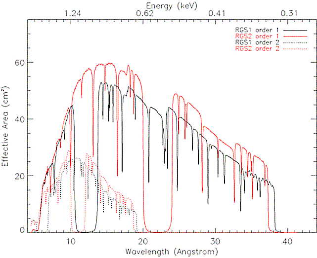
Fig. 84 displays the calculated effective area of both RGS units together, and Fig. 85 the individual RGS1 and RGS2 effective areas overlaid one on top of the other. The calculations have been performed taking into account all the factors listed above.

**Figure 84:** *The effective area of both RGS units combined as a function of energy and wavelength (top and bottom horizontal scales, respectively). See text for detailed explanations.*
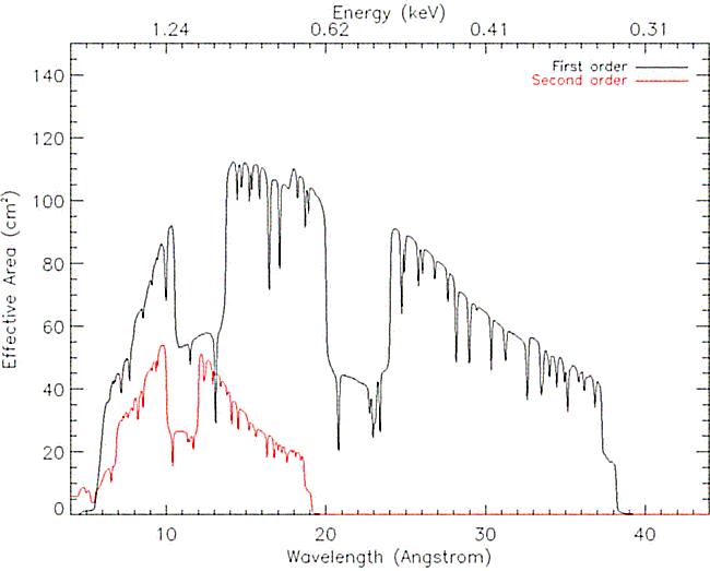$\begin{figure} \begin{center} \epsfig{file=figs/rgs_specarea2.eps,width=0.8\hsize,angle=0} \end{center} \end{figure}$

**Figure 85:** *The effective areas of both RGS units separately as a function of energy and wavelength (top and bottom horizontal scales, respectively). See text for detailed explanations.*
$\begin{figure} \begin{center} \epsfig{file=figs/rgs_specarea1.eps,width=0.8\hsize,angle=0} \end{center} \end{figure}$

Some clear features can be identified from these figures:

the effective area has broad gaps due to the inoperative CCDs.
the efficiency around chip boundaries does not drop sharply nor completely decreases to zero. This is due to the scattering causing photons with wavelengths corresponding to the passive areas being redistributed into non-passive areas. The amplitude of this sensitivity is strongly dependent on the selection mask in CCD PI versus dispersion coordinate space.
the total effective area of both RGS added in Fig. 84 shows several of these chip boundaries, as the alignment of the RGS cameras is such that the inter-chip gaps do not coincide in wavelength.
a similar effect of lower area as with the inter-chip gaps can be seen at wavelengths equivalent to bad columns, but there it is less pronounced.
absorption edges are due to the existence of passive layers in the X-ray path consisting of the following atoms: Si (6.74 Å), Al (7.95 Å), Mg (9.51 Å), F (17.80 Å) and O (22.83 Å)
apparent oscillations with small amplitude of the effective area are due to data selections by regions that are defined as polygons across the surface of binned two dimensional data (cross dispersion versus dispersion angle and CCD energy versus dispersion angle). The fact that pixels of these binned images are selected discretely, gives rise to small scale variations of the selected area within the region. This is seen as oscillations of the detection efficiency. This is not a problem, nor is it an additional uncertainty of the response, as these data selection effects are properly included in the response generation.

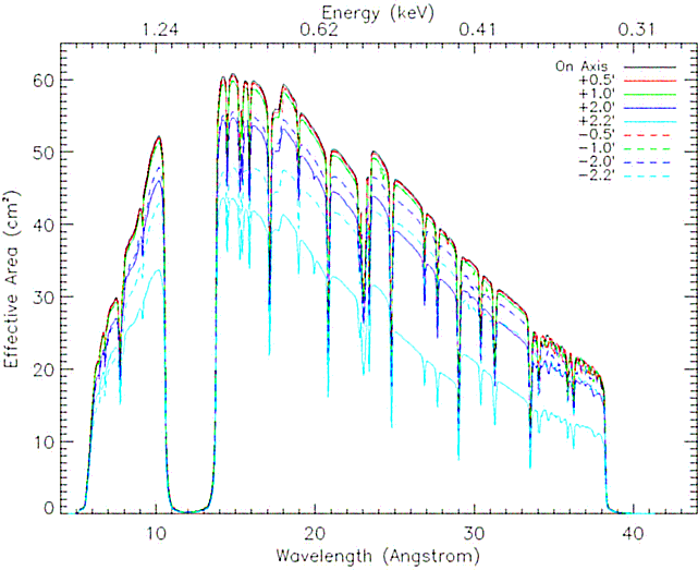
Fig. 86 shows the effective area as a function of the off-axis cross dispersion angle. The ratio of the median off-axis effective area to the on-axis values decreases from 0.994 at $\pm$ 0 $^\prime$ .5 to 0.83 and 0.60 at -2 $^\prime$ .2 and +2 $^\prime$ .2, respectively.

**Figure 86:** *The RGS1 effective area as a function of cross dispersion off-axis angle.*
$\begin{figure} \begin{center} \epsfig{file=figs/rgs_offaxis.ps,width=0.8\hsize,angle=0} \end{center} \end{figure}$

European Space Agency - XMM-Newton Science Operations Centre