Next: 3.5.6 OM brightness and dose limits Up: 3.5 OPTICAL MONITOR (OM) Previous: 3.5.4 Optical/UV point spread function of the OM and tracking
Both, Fig. 106 and Table 20,
provide the expected
count rate of the OM, in counts per second, for 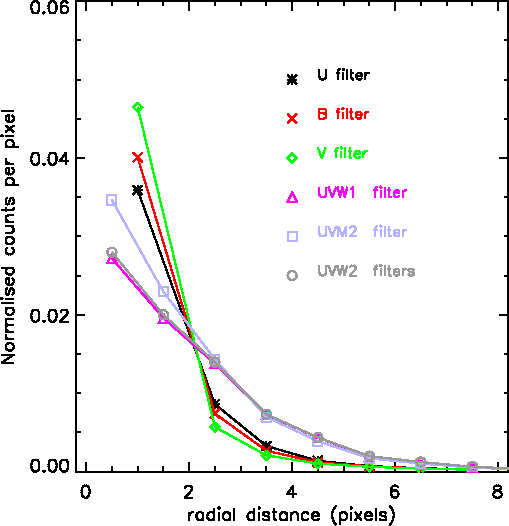 mag stars of
various types, with the different filters introduced above. These numbers
were obtained under the assumption of a perfect detector, i.e., free of
deadtime and coincidence loss, and without time sensitivity degradation,
and with an aperture radius of
mag stars of
various types, with the different filters introduced above. These numbers
were obtained under the assumption of a perfect detector, i.e., free of
deadtime and coincidence loss, and without time sensitivity degradation,
and with an aperture radius of  (
( ) for optical (UV) filters.
| Filter | B0 | A0 | F0 | G0 | G2 | K0 | M0 | WD |
| V | 1555 | 1510 | 1473 | 1473 | 1495 | 1452 | 1392 | 1412 |
| B | 6190 | 5272 | 3805 | 3010 | 2577 | 2289 | 1337 | 4454 |
| U | 8533 | 2216 | 1486 | 1119 | 966 | 444 | 178 | 4667 |
| UVW1 | 5647 | 958 | 366 | 218 | 182 | 29.1 | 17.4 | 3093 |
| UVM2 | 2276 | 316 | 39.3 | 8.69 | 5.54 | 0.436 | 0.032 | 1174 |
| UVW2 | 950 | 126 | 11.1 | 2.06 | 1.19 | 0.112 | 0.069 | 561 |
The numbers listed in Table 20 can be used to calculate the perfect detector count rates of stars of given magnitude by the formula
where  is the count rate of an mag star of the same
spectral type as the target, and
is the count rate of an mag star of the same
spectral type as the target, and  and
and  are the
  and
the count rate of the target of interest, respectively.
and
the count rate of the target of interest, respectively.
However, OM deadtime and coincidence losses must be taken into account, for instance using SAS.
For the 20th magnitude stars in Fig. 106 and
Table 20, OM coincidence losses are
negligible. Losses become significant for a point source
at a count rate of about 10 counts s (about 10% coincidence) for a full frame exposure.
The correction is approximated by the following formula:
is the count rate of incident photons from
equation (3),  is the actual measured
count rate,
is the actual measured
count rate,  is the CCD frametime in units of seconds and
 the frametransfer time in the same units (0.1740 ms).
The frametime is a function of the OM science window
configuration, as described in § 3.5.2.
the frametransfer time in the same units (0.1740 ms).
The frametime is a function of the OM science window
configuration, as described in § 3.5.2.
An optimum aperture radius of was found to be
the radius at which the loss correction formula is self
consistent. At this radius the accuracy of the coincidence loss correction
is at a level of 5% between different frametimes.
The validity range of the coincidence loss correction can be obtained from eq. 4 as a function of the frametime, whose maximum value (11.04 ms) occurs for full frame exposures, high or low resolution, where the whole detector is used. In windowed exposures the frametime varies from about 5 to 10 ms. For this reason the maximum measured count rates that can be reliably corrected are in the range of a few hundreds counts per second. Higher rates (1000 cts/s) may not damage the detector, but are scientifically useless.
We give in Table 21 coincidence loss corrected rates for limit high measured rates. The table gives the maximum measurable rate for each given value of frametime (1 count per frametime) and the corresponding corrected values for the maximum rate minus 0.01 and 0.001 c/s. For these high rates we obtain correction factors of 10, and very small differences in count rate produce variations in the corrected rates of more than 20%.
| Frametime | Maximum | Corrected rate | Corrected rate |
| measured rate | max-0.01 | max-0.001 | |
| (ms) | (c/s) | (c/s) | (c/s) |
| 5 | 200 | 2052 | 2531 |
| 7 | 143 | 1402 | 1739 |
| 9 | 111 | 1056 | 1317 |
| 11 | 91 | 842 | 1054 |
The coincidence loss correction implemented in SAS (from version 14) sets a validity limit at a rate of 0.97 counts per frametime (source+background). Within this limit, the correction error is less than 2%. This corresponds to about 700 and 300 source+background corrected counts for frametimes of 5 and 11 ms, respectively. For values higher than 0.97, the source counts are not corrected by SAS, and therefore, the conversion to magnitudes and fluxes are not applied. The produced source list contains only the measured count rate and position for these sources.
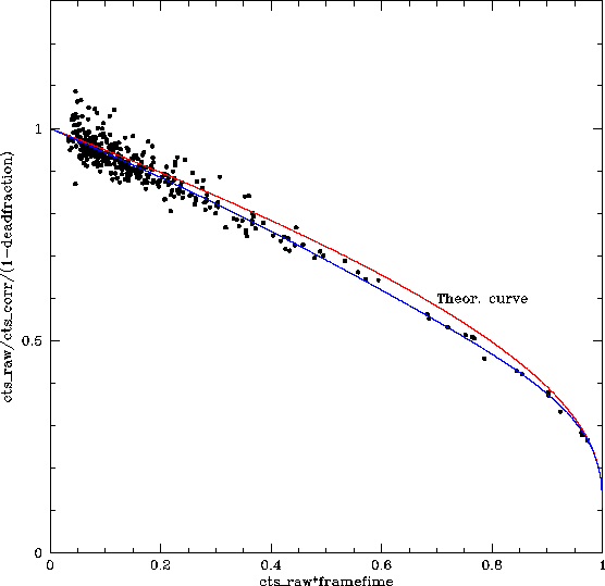
In Fig. 107, a comparison between formula (4) and the inflight instrument performance is shown.
 |
radius for optical filters and for UV) on which the
OM photometric calibration is based. If we consider that detections can
be obtained in the very few pixels in the core of the PSF, since the total
background is then lower, the limit would be about one magnitude fainter.
| Filter | Spectral type | ||||
| B0 | A0 | G0 | K0 | WD | |
| V | 19.8 | 19.8 | 19.7 | 19.7 | 19.7 |
| B | 21.0 | 20.8 | 20.2 | 19.9 | 20.6 |
| U | 21.8 | 20.4 | 19.6 | 18.6 | 21.2 |
| UVW1 | 21.1 | 19.2 | 17.6 | 15.4 | 20.5 |
 =10 mag solar type star per
square degree. All magnitudes are in V filter.
=10 mag solar type star per
square degree. All magnitudes are in V filter.
Table 23 presents the limiting magnitudes derived from the photometric analysis of one of the OM calibration fields (HD5980, also observed from the ground). This can be considered as an extreme case because of the crowdedness of the field which increases the observed background by overlap of the PSF wings. This is why the obtained limits are brighter than the simulations of Table 22.
| Filter | Spectral type range | ||
| B0/A0 | A1/G3 | G4/M8 | |
| V | 19.5 | 19.4 | 19.4 |
| B | 20.6 | 19.8 | 19.3 |
| U | 20.2 | 19.4 | 18.6 |
A detailed study of the background sources in OM can be found in:
http://www.cosmos.esa.int/documents/332006/623312/MSSLbckgd_v6.pdf
http://www.cosmos.esa.int/documents/332006/623312/OMbackg05.pdf.
The expected levels of different external background radiation processes
in the optical/UV are tabulated in Table 24.
The background count rate in the OM is dominated by the zodiacal
light in the optical. In the far UV the intrinsic detector background
becomes important. Images are regularly taken with the blocked filter
and no LED illumination to measure the detector dark counts. The
mean OM dark count rate is 4.0
 counts s pixel.
The variation across the detector is
counts s pixel.
The variation across the detector is  9% , with a mainly radial
dependence, being highest in an annulus of about 8' radius and
lowest at the centre. Variations as a function of time are broadly cyclic, on a timescale of 11 years
(likely associated to the solar cycle), with a semi-amplitude of 23%. If a very bright star
is in the field of view, the dark rate can be up to
9% , with a mainly radial
dependence, being highest in an annulus of about 8' radius and
lowest at the centre. Variations as a function of time are broadly cyclic, on a timescale of 11 years
(likely associated to the solar cycle), with a semi-amplitude of 23%. If a very bright star
is in the field of view, the dark rate can be up to  60%
higher than normal, despite the use of the Blocked filter.
60%
higher than normal, despite the use of the Blocked filter.
| Background source | Occurrence | Count rate range |
Diffuse Galactic |
all directions | 2.14 -7.527 -7.527 |
Zodiacal |
longitude
 |
1.69-5.611 |
Average dark count rate |
all directions |
 |
arcsec ].
pixel]
].
pixel]
Artifacts can appear in the XMM-Newton OM images due to light being scattered within the detector. These have two causes: internal reflection of light within the detector window and reflection of the off-axis starlight and background light from part of the detector housing.
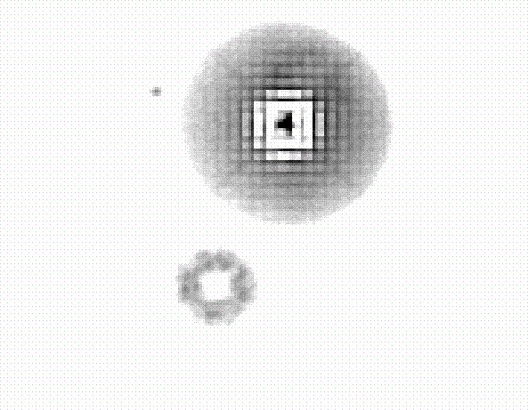
The first of these causes a faint, out of focus ghost image of a bright star, displaced in the radial direction away from the primary image (see Fig. 108).
 |
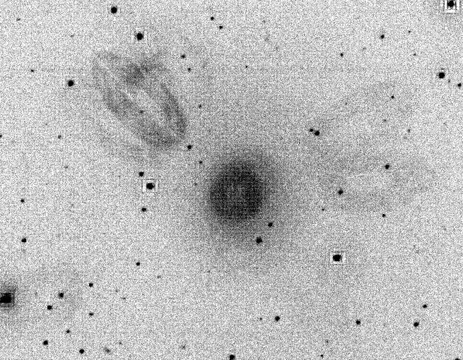
 to
to  off axis shine on the reflective ring
and form extended loops of emission radiating from the centre of the
detector (see Fig. 109).
off axis shine on the reflective ring
and form extended loops of emission radiating from the centre of the
detector (see Fig. 109).
 |
Similarly, there is an enhanced “ring” of emission near the centre of the detector due to diffuse background light falling on the ring. These features are less prominent when using UV filters, due to the lower reflectivity of UV light.
Figure 110 shows the low sensitivity patch produced by
an accidental observation of Jupiter in July 2017. This figure shows also the
"ring" mentioned before. The low sensitivity patch is oval with a size around
 pix
pix , equivalent to 1.4 square arcmin approximately. The
whole field is 17 arcmin in diameter.
, equivalent to 1.4 square arcmin approximately. The
whole field is 17 arcmin in diameter.
 |
European Space Agency - XMM-Newton Science Operations Centre