XMM-Newton Users Handbook

3.3.2 Science modes of the EPIC cameras

The EPIC cameras allow several modes of data acquisition. Note that in the case of MOS the outer ring of 6 CCDs remain in standard imaging mode while the central MOS CCD can be operated separately. Thus all CCDs are gathering data at all times, independent of the choice of operating mode. The pn camera CCDs can be operated in common modes in all quadrants for Full Frame, Extended Full Frame and Large Window mode, or just with one single CCD (CCD number 4 in Fig. 22) for Small Window, Timing and Burst mode.

1. “Full Frame” and “Extended Full Frame” (pn only)

   In this mode, all pixels of all CCDs are read out and thus the full FOV is covered.

2. “Partial Window”

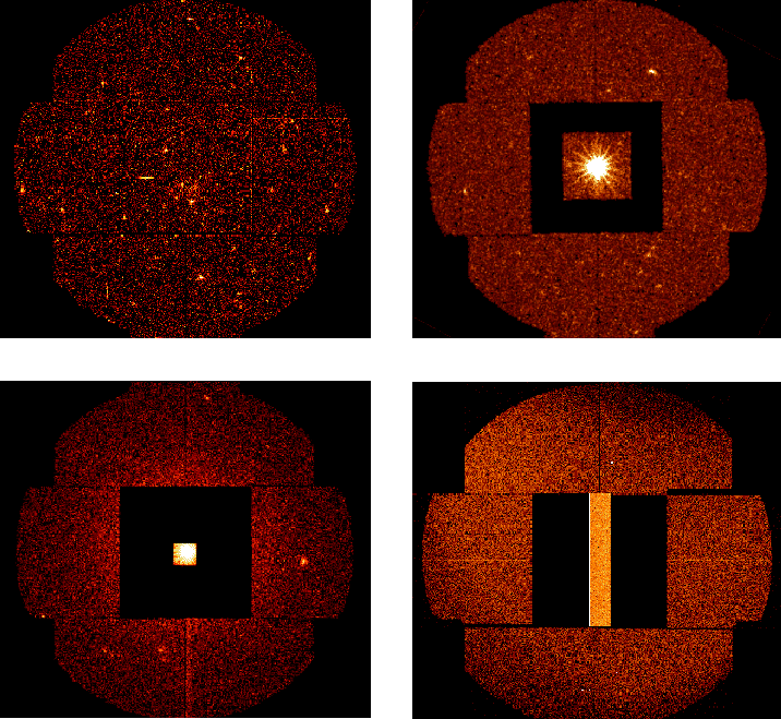
   a) MOS

   In a Partial Window mode the central CCD of both MOS cameras can be operated in a different mode of science data acquisition, reading out only part of the CCD chip.

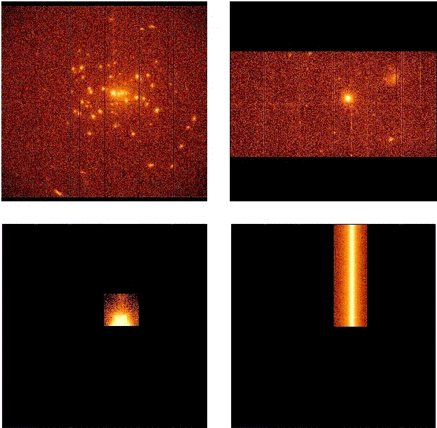
   b) pn

   In Large Window mode only half of the area in all 12 CCDs is read out, whereas in Small Window mode only a part of CCD number 4 is used to collect data. Note that the pn camera in these windowed modes is operated in such a way that non-read regions of the CCDs are exposed to the sky so that bright sources in these "dark" areas might still affect the observation.

3. “Timing”

   a) MOS + pn

   In the Timing mode, spatial information is maintained only in one dimension, along the column (RAWX) axis. For pn, the full width of CCD4 is active, whereas for MOS the active area is reduced to about 100 columns around the boresight. Along the row direction (RAWY axis), spatial information is lost due to continuous shifting and collapsing of rows to be read out at high speed. Since the 2 MOS cameras orientations differ by 90 degrees, the “imaging” direction in the 2 MOS are perpendicular to each other.

   b) pn only

   A special flavour of the Timing mode of the EPIC pn camera is the “Burst” mode, which offers very high time resolution, but has a very low duty cycle of 3%.

The most important characteristics of the EPIC science modes (time resolution and count rate capability) are tabulated in Table 3. Fig. 23 and Fig. 24 show the active CCD areas for the different pn and MOS readout modes, respectively.

Table 3: Basic numbers for the science modes of EPIC

MOS (central CCD; pixels) [1 pixel = 1.1"]	Time resolution	Live time$^1$ [%]	Max. count rate$^2$ diffuse$^3$ (total) [s$^{-1}$]	Max. count rate$^2$ (flux) point source [s$^{-1}$] ([mCrab]$^4$)
Full frame (600$\times$600)	2.6 s	100.0	150	0.50 (0.17)
Large window (300$\times$300)	0.9 s	99.5	110	1.5 (0.49)
Small window (100$\times$100)	0.3 s	97.5	37	4.5 (1.53)
Timing uncompressed (100$\times$600)	1.75 ms	100.0	N/A	100 (35)
pn (array or 1 CCD; pixels) [1 pixel = 4.1"]	Time resolution	Live time$^1$ [%]	Max. count rate$^2$ diffuse$^3$ (total) [s$^{-1}$]	Max. count rate$^2$ (flux) point source [s$^{-1}$] ([mCrab]$^4$)
Full frame$^5$ (376$\times$384)	73.4 ms	99.9	1000(total)	2 (0.23)
Extended full frame$^{5,6}$ (376$\times$384)	199.1 ms	100.0	370	0.7 (0.09)
Large window (198$\times$384)	47.7 ms	94.9	1500	3 (0.35)
Small window (63$\times$64)	5.7 ms	71.0	12000	25 (3.25)
Timing (64$\times$200)	0.03 ms	99.5	N/A	800 (85)
Burst (64$\times$180)	7 $\mu$s	3.0	N/A	60000 (6300)

Notes to Table 3:
1) Ratio between the time interval during which the CCD is collecting X-ray events (integration time, including time needed to shift events towards the readout) and the frame time (which in addition includes time needed for the readout of the events).
2) “Maximum” to avoid deteriorated response due to photon pile-up (see § 3.3.9 and XMM-SOC-CAL-TN-0200, available at http://www.cosmos.esa.int/web/xmm-newton/calibration-documentation) and X-ray loading (see 2nd point in § 3.3.6). These count rates include background. Note that telemetry limitations are in some cases more stringent than the pile-up constraints. For the MOS cameras the maximum count rates are about 115 counts/s for Full Window and Partial Window imaging modes and 230 counts/s for Timing mode. The pn telemetry limit is approximately 600 counts/s for the imaging modes and approximately 450 counts/s for the Timing mode. If the rate is higher, then the so-called counting mode is triggered and for some time the science data are lost. See also § 4.3.1 on the EPIC bright source avoidance. For sources with very soft spectra a factor of 2-3 lower maximum incident flux limits are recommended, while maximum count rates remain unchanged, see § 3.3.9. Despite the pile-up threshold being very similar in EPIC-pn Full Frame and Large Window modes, there are two intrinsic advantages of the latter which may compensate the loss of field-of-view: a) the significantly lower level of out-of-time events (0.16% versus $>$6%); b) the larger dynamical range in optical magnitude within which optical loading does not affect the data.
3) Values are representative of bright objects that are extended on scales much larger than the PSF core. In case of assumed homogeneous illumination on the CCD, a 1% pile-up limit for MOS is reached for a flux of 1 event per 900 pixels per frame.
4) Conventionally, it is assumed that 1 mCrab = $2.4\times10^{-11}$ erg s$^{-1}$ cm$^{-2}$ (in the energy range 2-10 keV).
5) The first 12 rows at the readout-node are not transmitted to ground (are set to “bad”, equivalent to “bad pixels”).
6) “Extended” means that the image collection time (i.e. the frame time) is longer than in the normal Full Frame mode.

Figure 23: Operating modes for the pn-CCD camera. Top left: Full Frame and Extended Full Frame mode; top right: Large Window mode; bottom left: Small Window mode, and bottom right: Timing mode. The Burst mode is different from the Timing mode as the source position is not read out, i.e. rows 181-200 will be dark.

Figure 24: Operating modes for the MOS-CCD cameras. Top left: Full Frame mode; top right: Large Window mode; bottom left: Small Window mode, and bottom right: Timing mode. In Timing mode, the X axis of the central CCD is the projected image of the source, and has thus true spatial information; the Y axis does not carry any spatial information but is a measure of time, with roll-over of 1024 time-units in the figure shown.

The count rate limitations are defined for a 2.5% flux loss (see § 3.3.9 and XMM-SOC-CAL-TN-0200 for details on pile-up) in point like sources. This level entails a $<$1% spectral distortion, which in this case is defined as the complement to 1 of the ratio between two measured count rates: the count rate of good patterns originated exclusively by one individual photon and the count rate of good patterns originated by all events. Early estimates of spectral fitting errors without any response matrix corrections show that a doubling of these count rates could lead to systematic errors greater than the nominal calibration accuracies. The Pile-up can be alleviated by excising the PSF core at the penalty of losing overall flux, but retaining spectral fitting integrity, modulo the accuracy in the calibration of the Point Spread Function wings.

For sources with very soft spectra, a factor of 2-3 lower maximum incident flux limits are recommended, while maximum count rates remain unchanged, see § 3.3.9. For the pn camera also for point sources with hard spectra (power law photon index $\alpha < 2$) lower count rate limits should be applied, in order to avoid X-ray loading (see XMM-SOC-CAL-TN-0050, available from http://www.cosmos.esa.int/web/xmm-newton/calibration-documentation). For $\alpha$=1.5 and 1.0 the maximum count rate limits given in Table 3 should be reduced by factors 2 and 4, respectively.

One of the major differences between the two types of camera is the high time resolution of the pn. With this camera high-speed photometry of rapidly variable targets can be conducted, down to a minimum integration time of 30 (7) $\mu$s in the Timing (Burst) mode.

The SAS task epatplot allows users to have a qualitative estimate of the level of pile-up affecting an input event list by comparing the observed and expected distributions of event PATTERNs. Users are referred to the description of this task in the SAS documentation (see also § 3.3.9 for details on pile-up).